Markets and Measurement II
Materials for class on Wednesday, January 10, 2018
Contents
Slides
Download the slides from today’s lecture.

Adjusting for inflation
Indicators
Adjusting for inflation
\[ \text{Real GDP} = \frac{\text{Nominal GDP}}{\text{Price Index / 100}} \]
- Worksheet we created in class
- Or, use the BLS’s CPI inflation calculator
Measuring inequality with Gini coefficients
Calculating Gini coefficients with R is trivial with the ineq package—create a vector of incomes and feed it into ineq(). Here’s what you do for a fictional country with the following incomes:
| Person | Income |
|---|---|
| 1 | $10,000 |
| 2 | $20,000 |
| 3 | $50,000 |
| 4 | $100,000 |
| 5 | $200,000 |
## [1] 0.4842105There are other types of inequality measures too. The default is Gini, but if you look at the documentation of ineq() with ?ineq, you can see the others.
You can plot the Lorenz curve easily too:
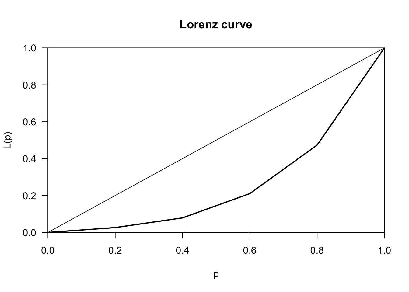
Alternatively you can extract the Lorenz curve that’s returned from Lc() and use ggplot2 to create a nicer plot:
library(tidyverse)
# This file is on GitHub at https://github.com/andrewheiss/econw18.classes.andrewheiss.com/blob/master/lib/graphics.R
source(file.path(here::here(), "lib", "graphics.R")) # Load theme and colors
lorenz <- Lc(incomes)
plot_data <- data_frame(prop_population = lorenz$p,
prop_income = lorenz$L)
plot_labels <- tribble(
~x, ~y, ~label,
0.6, 0.4, "A",
0.8, 0.2, "B"
)
ggplot(plot_data, aes(x = prop_population, y = prop_income)) +
geom_line() +
geom_segment(x = 0, xend = 1, y = 0, yend = 1) +
geom_ribbon(aes(ymax = prop_population, ymin = prop_income), fill = nord_red) +
geom_ribbon(aes(ymax = prop_income, ymin = 0), fill = "grey80") +
geom_point(size = 2) +
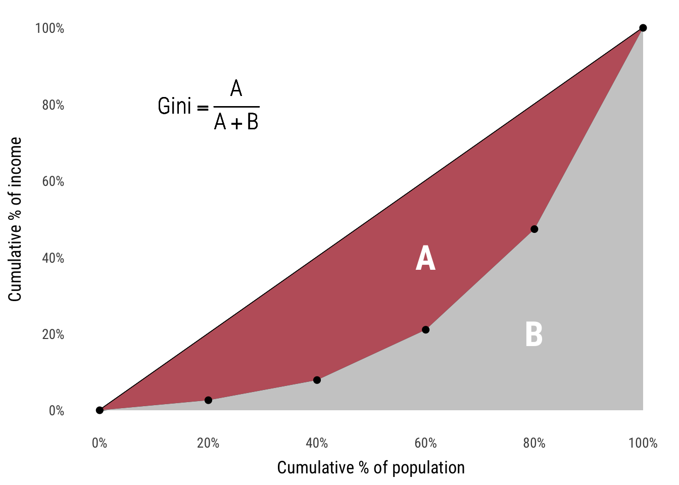
geom_text(x = 0.2, y = 0.8, label = "Gini == frac(A, A + B)", parse = TRUE,
size = 6, family = "Roboto Condensed Light") +
geom_text(data = plot_labels, aes(x = x, y = y, label = label),
color = "white", size = 9, family = "Roboto Condensed Bold") +
labs(x = "Cumulative % of population", y = "Cumulative % of income") +
scale_x_continuous(labels = scales::percent, breaks = seq(0, 1, 0.2)) +
scale_y_continuous(labels = scales::percent, breaks = seq(0, 1, 0.2)) +
theme_econ(13) +
theme(panel.grid = element_blank())